Pytorch官方教程(一)—A 60 Minute Biltz
What is Pytorch?
Pytorch 是 python 针对两类受众的一个基础科学计算包:
- 替代 numpy 使用 GPU 的功能
- 为深度学习研究者提供最大灵活性和速度的框架
Tensors
Tensors 类似于 Numpy 中的 ndarrays,另外 Tensors 还可以使用 GPU 加速计算。
from __future__ import print_function
import torch
创建一个 5x3 的矩阵,未初始化
x = torch.empty(5, 3)
print(x)
tensor([[-1.2316e-14,  4.5688e-41, -1.2316e-14],
        [ 4.5688e-41, -1.5579e-14,  4.5688e-41],
        [ 1.1270e+17,  3.0746e-41,  1.1270e+17],
        [ 3.0746e-41, -1.7668e-14,  4.5688e-41],
        [-1.7058e-14,  4.5688e-41,  9.4459e+37]])
创建一个随机初始化的矩阵
x = torch.rand(5, 3)
print(x)
tensor([[ 0.9167,  0.4915,  0.5527],
        [ 0.1328,  0.3441,  0.7412],
        [ 0.0099,  0.3940,  0.4559],
        [ 0.6498,  0.2526,  0.4083],
        [ 0.2442,  0.0457,  0.4149]])
创建一个 0 矩阵,dtype = long
x = torch.zeros(5, 3, dtype=torch.long)
print(x)
tensor([[ 0,  0,  0],
        [ 0,  0,  0],
        [ 0,  0,  0],
        [ 0,  0,  0],
        [ 0,  0,  0]])
直接用数据创建 tensor
x = torch.tensor([5.5, 3])
print(x)
tensor([ 5.5000, 3.0000])
在已有的 tensor 上创建 tensor。这中方式将重用输入 tensor 的属性,例如 dtype,除非用户提供了新的值。
x = x.new_ones(5, 3, dtype=torch.double)      # new_* methods take in sizes
print(x)

x = torch.randn_like(x, dtype=torch.float)    # override dtype!
print(x)                                      # result has the same size
tensor([[ 1.,  1.,  1.],
        [ 1.,  1.,  1.],
        [ 1.,  1.,  1.],
        [ 1.,  1.,  1.],
        [ 1.,  1.,  1.]], dtype=torch.float64)
tensor([[-1.2265, -0.9197,  0.6174],
        [ 0.6637, -1.7571, -0.0190],
        [ 1.4778,  0.9150, -0.9859],
        [ 2.4320,  1.1956, -1.1652],
        [ 0.7804,  0.9591,  0.6425]])
获取 tensor 大小
print(x.size())
torch.Size([5, 3])
Note:
torch.Size 实际上是个 tuple,因此它支持 tuple 的所有运算。
Operations
有多种运算语法。在下面的例子中,我们看一下加法运算。
加法:语法1
y = torch.rand(5, 3)
print(x + y)
tensor([[-0.6736, -0.3655,  0.9713],
        [ 1.1350, -1.3696,  0.8927],
        [ 1.6723,  1.2142, -0.2705],
        [ 3.1239,  1.9089, -0.5061],
        [ 0.9300,  1.5780,  0.8623]])
加法:语法2
print(torch.add(x, y))
tensor([[-0.6736, -0.3655,  0.9713],
        [ 1.1350, -1.3696,  0.8927],
        [ 1.6723,  1.2142, -0.2705],
        [ 3.1239,  1.9089, -0.5061],
        [ 0.9300,  1.5780,  0.8623]])
加法:提供一个输出 tensor 作为 argument
result = torch.empty(5, 3)
torch.add(x, y, out=result)
print(result)
tensor([[-0.6736, -0.3655,  0.9713],
        [ 1.1350, -1.3696,  0.8927],
        [ 1.6723,  1.2142, -0.2705],
        [ 3.1239,  1.9089, -0.5061],
        [ 0.9300,  1.5780,  0.8623]])
加法:in-place
# adds x to y
y.add_(x)
print(y)
tensor([[-0.6736, -0.3655,  0.9713],
        [ 1.1350, -1.3696,  0.8927],
        [ 1.6723,  1.2142, -0.2705],
        [ 3.1239,  1.9089, -0.5061],
        [ 0.9300,  1.5780,  0.8623]])
Note:
以 _ 结尾的运算都将改变原 tensor。例如: x.copy_(y), x.t_(), x 将会改变。
你可以使用类似 numpy 的索引,包含其所有附加功能。
print(x[:, 1])
tensor([-0.9197, -1.7571, 0.9150, 1.1956, 0.9591])
torch.view: resize/reshape tensor
x = torch.randn(4, 4)
y = x.view(16)
z = x.view(-1, 8)  # the size -1 is inferred from other dimensions
print(x.size(), y.size(), z.size())
torch.Size([4, 4]) torch.Size([16]) torch.Size([2, 8])
针对只有一个元素的 tensor,可以使用 .item() 得到 tensor 的值作为 python 数字。
x = torch.randn(1)
print(x)
print(x.item())
tensor([-0.1896])
-0.18955747783184052
NumPy Bridge
Torch Tensor 与 Numpy Array 的相互转换。Torch Tensor 与 Numpy Array 将共享他们的底层内存地址,更改一个将更改另一个。
Torch Tensor -> Numpy Array
a = torch.ones(5)
print(a)
b = a.numpy()
print(b)
tensor([ 1.,  1.,  1.,  1.,  1.])
[1. 1. 1. 1. 1.]
a.add_(1)
print(a)
print(b)
tensor([ 2.,  2.,  2.,  2.,  2.])
[2. 2. 2. 2. 2.]
Numpy Array -> Torch Tensor
import numpy as np

a = np.ones(5)
b = torch.from_numpy(a)
np.add(a, 1, out=a)
print(a)
print(b)
[2. 2. 2. 2. 2.]
tensor([ 2.,  2.,  2.,  2.,  2.], dtype=torch.float64)
所有在 CPU 上的 Tensors 除了 CharTensor 类型,都支持与 Numpy 的相互转换。
CUDA Tensors
Tensors 可以使用 .to 方法移到任何设备上。
# let us run this cell only if CUDA is available
# We will use ``torch.device`` objects to move tensors in and out of GPU
if torch.cuda.is_available():
    device = torch.device("cuda:0")          # a CUDA device object
    y = torch.ones_like(x, device=device)  # directly create a tensor on GPU
    x = x.to(device)                       # or just use strings ``.to("cuda")``
    z = x + y
    print(z)
    print(z.to("cpu", torch.double))       # ``.to`` can also change dtype together!
tensor([ 0.8104], device='cuda:0')
tensor([ 0.8104], dtype=torch.float64)
Autograd: Automatic Differentiation
在 pytorch 中,对于神经网络 autograd 是关键库。我们先简略的熟悉一下这个库,然后训练我们的第一个神经网络。
autograd 对于 Tensors 的所有运算提供了自动微分的功能。它是一个运行时定义的框架(动态计算图),这意味着反向传播由运行时的代码决定,并且每次迭代都可以不同。
Tensor
torch.Tensor 是这个包的关键类。如果将它的属性 .requires_grad 设置为 True,它开始追踪它的所有运算。完成计算时,调用 .backward(),所有的梯度计算将自动完成。tensor 的梯度存储在 .grad 属性中。
要阻止 tensor 追踪历史纪录,可以调用 .detach() 将其从计算历史纪录中分离出来,并防止将来的计算被追踪。要阻止追踪历史记录(使用内存),也可以使用 with torch.no_grad(): 将代码封装起来。当评估一个模型时,这是特别有帮助的,因为训练好的模型参数可能是 requires_grad=Ture,但评估模型不需要梯度。
还有一个类对实现自动微分非常重要 - Function。Tensor 和 Function 是相互连接的,并且创建了一个无环计算图。每个 Tensor 有一个 .grad_fn 属性,引用创建 Tensor 的 Function(除了用户创建的 Tensors - 它的 grad_fn 是 None)。
对 Tensor 调用 .backward() 可以计算微分。如果 Tensor 是个标量(也就是说它的数据只有一个元素),backward()不需要指定任何参数。如果 Tensor 有多个元素,需指定匹配 tensor 形状的参数 gradient。
import torch
创建一个tensor,设置 requires_grad = True 用于追踪计算。
x = torch.ones(2, 2, requires_grad=True)
print(x)
tensor([[ 1.,  1.],
        [ 1.,  1.]])
对 tensor 进行运算
y = x + 2
print(y)
tensor([[ 3.,  3.],
        [ 3.,  3.]])
y 作为运算的结果被创建,因此它有 grad_fn 属性
print(y.grad_fn)
<AddBackward0 object at 0x7f5c7c0e8710>
对 y 进行更多的运算
z = y * y * 3
out = z.mean()
print(z, z.grad_fn)
print(out, out.grad_fn)
tensor([[ 27.,  27.],
        [ 27.,  27.]]) <MulBackward0 object at 0x7f5c7c0fa128>
tensor(27.) <MeanBackward1 object at 0x7f5c7c0fa198>
.requires_grad_( … ) 改变 Tensor 的 requires_grad 属性。requires_grad 的默认值为 False
a = torch.randn(2, 2)
a = ((a * 3) / (a - 1))
print(a.requires_grad)
a.requires_grad_(True)
print(a.requires_grad)
b = (a * a).sum()
print(b.grad_fn)
False
True
<SumBackward0 object at 0x7f5c7c0fa5f8>
Gradients
因为 out 只包含单个标量,因此 out.backward() 等同于 out.backward(torch.tensor(1.))。
out.backward()
打印梯度d(out)/dx
print(x.grad)
tensor([[ 4.5000,  4.5000],
        [ 4.5000,  4.5000]])
得到一个值为 4.5 的矩阵。用 ‘o’ 代表 Tensor out。我们有 $o = \frac{1}{4}\sum_i z_i$,$z_i = 3(x_i+2)^2$ 和 $z_i\bigr\rvert_{x_i=1} = 27$,所以,$\frac{\partial o}{\partial x_i} = \frac{3}{2}(x_i+2)$,所以 $\frac{\partial o}{\partial x_i}\bigr\rvert_{x_i=1} = \frac{9}{2} = 4.5$。
在数学上,一个向量函数 $\vec{y}=f(\vec{x})$,$\vec{y}$ 对 $\vec{x}$ 求得的微分是一个雅可比矩阵:
总体上讲,torch.autograd 是一个计算矢量雅可比矩阵乘积的引擎,即对于给定的向量 $v=\left(\begin{array}{cccc} v_{1} & v_{2} & \cdots & v_{m}\end{array}\right)^{T}$ 计算乘积 $v^{T}\cdot J$。如果 $v$ 是一个标量函数的梯度 $l=g\left(\vec{y}\right)$,即 $v=\left(\begin{array}{ccc}\frac{\partial l}{\partial y_{1}} & \cdots & \frac{\partial l}{\partial y_{m}}\end{array}\right)^{T}$,根据链式法则,矢量雅可比矩阵的乘积将会是 $l$ 对 $\vec{x}$ 的微分。
($v^{T}\cdot J$ 给出一个行向量,可以通过 $J^{T}\cdot v $ 将其视为列向量。)
矢量雅可比矩阵乘积的这个特性使得将外部梯度输入到具有非标量输出的模型中非常方便。
x = torch.randn(3, requires_grad=True)

y = x * 2
while y.data.norm() < 1000:
    y = y * 2

print(y)
tensor([ -740.1835, 1359.2710, 530.6011])
在这种情况下 y 不再是标量。torch.autograd 不能直接计算出这个雅可比矩阵,不过如果如果我们只想得到矢量雅可比矩阵的乘积,只需将向量作为参数传递给 backward。
v = torch.tensor([0.1, 1.0, 0.0001], dtype=torch.float)
y.backward(v)

print(x.grad)
tensor([ 102.4000, 1024.0000, 0.1024])
你还可以通过使用 torch.no_grad() 来封装代码,阻止属性为 .requires_grad = True 的 tensor 从追踪的历史纪录中自动微分:
print(x.requires_grad)
print((x ** 2).requires_grad)

with torch.no_grad():
    print((x ** 2).requires_grad)
True
True
False
Neural Networks
可使用 torch.nn 包搭建神经网络。
现在你已经了解了 autograd,nn 依赖于 autograd 构建模型及其微分。一个 nn.Module 包含多个层,返回 output 的 forward(input) 方法。
神经网络典型的训练过程:
- 定义一个有可学参数(或 weights)的神经网络
- 遍历输入数据集
- 把数据集输入神经网络
- 计算损失函数(与正确输出的差距)
- 将梯度反向传播到网络参数
- 更新网络权重,典型的更新规则:weight = weight - learning_rate * gradient
Define the network
import torch
import torch.nn as nn
import torch.nn.functional as F


class Net(nn.Module):

    def __init__(self):
        super(Net, self).__init__()
        # 1 input image channel, 6 output channels, 5x5 square convolution
        # kernel
        self.conv1 = nn.Conv2d(1, 6, 5)
        self.conv2 = nn.Conv2d(6, 16, 5)
        # an affine operation: y = Wx + b
        self.fc1 = nn.Linear(16 * 5 * 5, 120)
        self.fc2 = nn.Linear(120, 84)
        self.fc3 = nn.Linear(84, 10)

    def forward(self, x):
        # Max pooling over a (2, 2) window
        x = F.max_pool2d(F.relu(self.conv1(x)), (2, 2))
        # If the size is a square you can only specify a single number
        x = F.max_pool2d(F.relu(self.conv2(x)), 2)
        x = x.view(-1, self.num_flat_features(x))
        x = F.relu(self.fc1(x))
        x = F.relu(self.fc2(x))
        x = self.fc3(x)
        return x

    def num_flat_features(self, x):
        size = x.size()[1:]  # all dimensions except the batch dimension
        num_features = 1
        for s in size:
            num_features *= s
        return num_features


net = Net()
print(net)
Net(
  (conv1): Conv2d(1, 6, kernel_size=(5, 5), stride=(1, 1))
  (conv2): Conv2d(6, 16, kernel_size=(5, 5), stride=(1, 1))
  (fc1): Linear(in_features=400, out_features=120, bias=True)
  (fc2): Linear(in_features=120, out_features=84, bias=True)
  (fc3): Linear(in_features=84, out_features=10, bias=True)
)
只需定义前向传播函数,然后使用 autograd 自动完成反向传播函数(其中计算梯度),在前向传播函数中可以使用任何 Tensor 操作。
net.parameters()返回模型的可学习参数。
params = list(net.parameters())
print(len(params))
print(params[0].size())  # conv1's .weight
10
torch.Size([6, 1, 5, 5])
随机输入一个 32x32 矩阵。
input = torch.randn(1, 1, 32, 32)
out = net(input)
print(out)
tensor([[ 0.0993, -0.1024, -0.0992, -0.0034,  0.0570, -0.0229, -0.1167,
         -0.0303, -0.0810, -0.0111]])
将所有参数的梯度缓存清零,随机选取梯度进行反向传播。
net.zero_grad()
out.backward(torch.randn(1, 10))
NOTE
torch.nn 仅支持 mini-batch 格式。整个 torch.nn 包也仅支持 mini-batch 样本的输入,而非单个样本。例如,nn.Conv2d 接受一个 4 维 Tensor(nSamples x nChannels x Height x Width)。要输入单个样本,使用 input.unsqueeze(0) 增加 batch 维度。
Loss Function
损失函数用(output,target)对为输入,并计算输出与目标的差距。nn 包中有多种不同的损失函数。例如,nn.MSELoss 计算输入与目标的均方误差。
output = net(input)
target = torch.randn(10)  # a dummy target, for example
target = target.view(1, -1)  # make it the same shape as output
criterion = nn.MSELoss()

loss = criterion(output, target)
print(loss)
tensor(0.3910)
使用.grad_fn 属性沿着 loss 进行反向追踪,可得到计算图:
input -> conv2d -> relu -> maxpool2d -> conv2d -> relu -> maxpool2d<br>
-> view -> linear -> relu -> linear -> relu -> linear<br>
-> MSELoss<br>
-> loss
调用 loss.backward(),整个图是关于 loss 的微分,在图中所有 requires_grad=True 的 Tensor,他们的 .grad Tensor 将会累积梯度。
print(loss.grad_fn)  # MSELoss
print(loss.grad_fn.next_functions[0][0])  # Linear
print(loss.grad_fn.next_functions[0][0].next_functions[0][0])  # ReLU
<MseLossBackward object at 0x7fd7ca0ba1d0>
<AddmmBackward object at 0x7fd7ca0ba2b0>
<ExpandBackward object at 0x7fd7ca0ba1d0>
Backprop
loss.backward() 用于反向传播 loss error。
必须先清空现有的梯度,否则梯度将会累加到现有梯度上。
现在我们调用 loss.backward(),看一下 conv1’s bias 反向传播前后的梯度。
net.zero_grad()     # zeroes the gradient buffers of all parameters

print('conv1.bias.grad before backward')
print(net.conv1.bias.grad)

loss.backward()

print('conv1.bias.grad after backward')
print(net.conv1.bias.grad)
conv1.bias.grad before backward
tensor([ 0.,  0.,  0.,  0.,  0.,  0.])
conv1.bias.grad after backward
tensor(1.00000e-02 *
       [ 0.3780,  0.1624, -0.2881, -0.2887, -1.0177, -0.1864])
Update the weights
使用最简单的更新规则——SGD:weight = weight - learning_rate * gradient。也可以通过简单的 python 代码实现:
learning_rate = 0.01
for f in net.parameters():
    f.data.sub_(f.grad.data * learning_rate)
torch.optim 包封装了各种优化器:SGD, Nesterov-SGD, Adam, RMSProp, etc
import torch.optim as optim

# create your optimizer
optimizer = optim.SGD(net.parameters(), lr=0.01)

# in your training loop:
optimizer.zero_grad()   # zero the gradient buffers
output = net(input)
loss = criterion(output, target)
loss.backward()
optimizer.step()    # Does the update
Note
梯度缓存必须使用 optimizer.zero_grad() 手动置 0。
Training A Classifier
对于视觉数据集,torchvision 用于加载公开数据集,如 Imagenet, CIFAR10, MNIST等等,对于图像变换有 torchvision.datasets 和 torch.utils.data.DataLoader。
训练 CIFAR10 数据集,步骤:
- 用 torchvision 加载、正则化 CIFAR10 的训练集和测试集
- 定义一个卷积神经网络
- 定义损失函数
- 用训练集训练网络
- 用测试集测试网络
Loading and normalizing CIFAR10
import torch
import torchvision
import torchvision.transforms as transforms
torchvision 数据集输出的图片是 [0, 1] 的 PILImage,转换为 [-1, 1] 的 Tensor。
transform = transforms.Compose(
    [transforms.ToTensor(),
     transforms.Normalize((0.5, 0.5, 0.5), (0.5, 0.5, 0.5))])

trainset = torchvision.datasets.CIFAR10(root='./data', train=True,
                                        download=True, transform=transform)
trainloader = torch.utils.data.DataLoader(trainset, batch_size=4,
                                          shuffle=True, num_workers=2)

testset = torchvision.datasets.CIFAR10(root='./data', train=False,
                                       download=True, transform=transform)
testloader = torch.utils.data.DataLoader(testset, batch_size=4,
                                         shuffle=False, num_workers=2)

classes = ('plane', 'car', 'bird', 'cat',
           'deer', 'dog', 'frog', 'horse', 'ship', 'truck')
Downloading https://www.cs.toronto.edu/~kriz/cifar-10-python.tar.gz to ./data/cifar-10-python.tar.gz
Files already downloaded and verified
显示训练集的图片
import matplotlib.pyplot as plt
import numpy as np

# functions to show an image


def imshow(img):
    img = img / 2 + 0.5     # unnormalize
    npimg = img.numpy()
    plt.imshow(np.transpose(npimg, (1, 2, 0)))
    plt.show()


# get some random training images
dataiter = iter(trainloader)
images, labels = dataiter.next()

# show images
imshow(torchvision.utils.make_grid(images))
# print labels
print(' '.join('%5s' % classes[labels[j]] for j in range(4)))
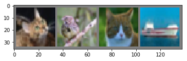
cat bird cat ship
Define a Convolutional Neural Network
import torch.nn as nn
import torch.nn.functional as F


class Net(nn.Module):
    def __init__(self):
        super(Net, self).__init__()
        self.conv1 = nn.Conv2d(3, 6, 5)
        self.pool = nn.MaxPool2d(2, 2)
        self.conv2 = nn.Conv2d(6, 16, 5)
        self.fc1 = nn.Linear(16 * 5 * 5, 120)
        self.fc2 = nn.Linear(120, 84)
        self.fc3 = nn.Linear(84, 10)

    def forward(self, x):
        x = self.pool(F.relu(self.conv1(x)))
        x = self.pool(F.relu(self.conv2(x)))
        x = x.view(-1, 16 * 5 * 5)
        x = F.relu(self.fc1(x))
        x = F.relu(self.fc2(x))
        x = self.fc3(x)
        return x


net = Net()
Define a Loss function and optimizer
使用交叉熵损失函数和 momentum SGD 优化器
import torch.optim as optim

criterion = nn.CrossEntropyLoss()
optimizer = optim.SGD(net.parameters(), lr=0.001, momentum=0.9)
Train the network
遍历输入迭代器,将输入传递给网络并优化。
for epoch in range(2):  # loop over the dataset multiple times

    running_loss = 0.0
    for i, data in enumerate(trainloader, 0):
        # get the inputs
        inputs, labels = data

        # zero the parameter gradients
        optimizer.zero_grad()

        # forward + backward + optimize
        outputs = net(inputs)
        loss = criterion(outputs, labels)
        loss.backward()
        optimizer.step()

        # print statistics
        running_loss += loss.item()
        if i % 2000 == 1999:    # print every 2000 mini-batches
            print('[%d, %5d] loss: %.3f' %
                  (epoch + 1, i + 1, running_loss / 2000))
            running_loss = 0.0

print('Finished Training')
[1,  2000] loss: 2.178
[1,  4000] loss: 1.852
[1,  6000] loss: 1.676
[1,  8000] loss: 1.597
[1, 10000] loss: 1.541
[1, 12000] loss: 1.481
[2,  2000] loss: 1.415
[2,  4000] loss: 1.382
[2,  6000] loss: 1.373
[2,  8000] loss: 1.349
[2, 10000] loss: 1.324
[2, 12000] loss: 1.308
Finished Training
Test the network on the test data
我们依据遍历了两遍训练集。我们检测一下网络学到了什么。我们通过预测神经网络输出的类标签来检查,并与 ground-truth 对比一下。如果预测是正确的,将样本添加到正确预测的列表中。
显示测试集图片
dataiter = iter(testloader)
images, labels = dataiter.next()

# print images
imshow(torchvision.utils.make_grid(images))
print('GroundTruth: ', ' '.join('%5s' % classes[labels[j]] for j in range(4)))
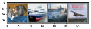
GroundTruth: cat ship ship plane
通过神经网络预测这些图片
outputs = net(images)
输出是这10类的概率。输出的值越大,这个类别的概率越高。我们看一下概率最高的类别。
_, predicted = torch.max(outputs, 1)

print('Predicted: ', ' '.join('%5s' % classes[predicted[j]]
                              for j in range(4)))
Predicted: cat car car ship
网络在整个测试集上的效果
correct = 0
total = 0
with torch.no_grad():
    for data in testloader:
        images, labels = data
        outputs = net(images)
        _, predicted = torch.max(outputs.data, 1)
        total += labels.size(0)
        correct += (predicted == labels).sum().item()

print('Accuracy of the network on the 10000 test images: %d %%' % (
    100 * correct / total))
Accuracy of the network on the 10000 test images: 53 %
按类别查看测试集的效果
class_correct = list(0. for i in range(10))
class_total = list(0. for i in range(10))
with torch.no_grad():
    for data in testloader:
        images, labels = data
        outputs = net(images)
        _, predicted = torch.max(outputs, 1)
        c = (predicted == labels).squeeze()
        for i in range(4):
            label = labels[i]
            class_correct[label] += c[i].item()
            class_total[label] += 1


for i in range(10):
    print('Accuracy of %5s : %2d %%' % (
        classes[i], 100 * class_correct[i] / class_total[i]))
Accuracy of plane : 40 %
Accuracy of   car : 73 %
Accuracy of  bird : 42 %
Accuracy of   cat : 39 %
Accuracy of  deer : 44 %
Accuracy of   dog : 53 %
Accuracy of  frog : 62 %
Accuracy of horse : 44 %
Accuracy of  ship : 69 %
Accuracy of truck : 66 %
Training on GPU
就像把 Tensor 移到 GPU 上,也可以把网络移到 GPU 上。
定义默认设备为 cuda
device = torch.device("cuda:0" if torch.cuda.is_available() else "cpu")

# Assuming that we are on a CUDA machine, this should print a CUDA device:

print(device)
cuda:0
本节剩余部分假设 device 是 cuda
然后这个方法将递归遍历所有模块并将其参数和缓存区转换为 cuda Tensor
net.to(device)
Net(
  (conv1): Conv2d(3, 6, kernel_size=(5, 5), stride=(1, 1))
  (pool): MaxPool2d(kernel_size=2, stride=2, padding=0, dilation=1, ceil_mode=False)
  (conv2): Conv2d(6, 16, kernel_size=(5, 5), stride=(1, 1))
  (fc1): Linear(in_features=400, out_features=120, bias=True)
  (fc2): Linear(in_features=120, out_features=84, bias=True)
  (fc3): Linear(in_features=84, out_features=10, bias=True)
)
还必须在每一步将输入和标签传送到 GPU 上
inputs, labels = inputs.to(device), labels.to(device)
Data Parallelism
使用 DataParallel 在多 GPU 上并行。
Pytorch 使用 GPU 是非常简单的。也可以把模型移到 GPU 上:
device = torch.device("cuda:0")
model.to(device)
之后,把所有的 tensor 拷贝到 GPU 上:
mytensor = my_tensor.to(device)
调用 my_tensor.to(device) 返回一个新的 在 GPU 上的 my_tensor 的副本,而不是重写 my_tensor。你需要先给分配一个新的 tensor 再在 GPU 上使用这个 tensor。
pytorch 默认使用一个 GPU 进行网络的正向传播和反向传播。使用 DataParallel 在多个 GPU 上并行模型:
model = nn.DataParallel(model)
Imports and parameters
import torch
import torch.nn as nn
from torch.utils.data import Dataset, DataLoader

# Parameters and DataLoaders
input_size = 5
output_size = 2

batch_size = 30
data_size = 100
Device
device = torch.device("cuda:0" if torch.cuda.is_available() else "cpu")
Dummy DataSet
创建虚拟数据集。仅需要定义 getitem
class RandomDataset(Dataset):

    def __init__(self, size, length):
        self.len = length
        self.data = torch.randn(length, size)

    def __getitem__(self, index):
        return self.data[index]

    def __len__(self):
        return self.len

rand_loader = DataLoader(dataset=RandomDataset(input_size, data_size),
                         batch_size=batch_size, shuffle=True)
Simple Model
在这个例子中,我们的模型只有输入层、线性运算和输出。可以在任何模型(CNN, RNN, Capsule Net etc.)中使用 DataParallel。
我们在模型放置了一个 print 语句来监视输入、输出 tensor 的大小。
class Model(nn.Module):
    # Our model

    def __init__(self, input_size, output_size):
        super(Model, self).__init__()
        self.fc = nn.Linear(input_size, output_size)

    def forward(self, input):
        output = self.fc(input)
        print("\tIn Model: input size", input.size(),
              "output size", output.size())

        return output
Create Model and DataParallel
首先,创建一个模型实例,检查是否有多个 GPU。如果有多个 GPU 可以使用 nn.DataParallel。然后用 model.to(device) 把模型放到 GPU 上。
model = Model(input_size, output_size)
if torch.cuda.device_count() > 1:
  print("Let's use", torch.cuda.device_count(), "GPUs!")
  # dim = 0 [30, xxx] -> [10, ...], [10, ...], [10, ...] on 3 GPUs
  model = nn.DataParallel(model)

model.to(device)
Let's use 4 GPUs!


DataParallel(
  (module): Model(
    (fc): Linear(in_features=5, out_features=2, bias=True)
  )
)
Run the Model
查看输入、输出 Tensor 的大小
for data in rand_loader:
    input = data.to(device)
    output = model(input)
    print("Outside: input size", input.size(),
          "output_size", output.size())
	In Model: input size torch.Size([8, 5]) output size torch.Size([8, 2])
	In Model: input size torch.Size([8, 5]) output size torch.Size([8, 2])
	In Model: input size torch.Size([6, 5]) output size torch.Size([6, 2])
	In Model: input size torch.Size([8, 5]) output size torch.Size([8, 2])
Outside: input size torch.Size([30, 5]) output_size torch.Size([30, 2])
	In Model: input size torch.Size([8, 5]) output size torch.Size([8, 2])
	In Model: input size torch.Size([8, 5]) output size torch.Size([8, 2])
	In Model: input size torch.Size([8, 5]) output size torch.Size([8, 2])
	In Model: input size torch.Size([6, 5]) output size torch.Size([6, 2])
Outside: input size torch.Size([30, 5]) output_size torch.Size([30, 2])
	In Model: input size torch.Size([3, 5]) output size torch.Size([3, 2])
	In Model: input size torch.Size([3, 5]) output size torch.Size([3, 2])
	In Model: input size torch.Size([3, 5]) output size torch.Size([3, 2])
	In Model: input size torch.Size([1, 5]) output size torch.Size([1, 2])
Outside: input size torch.Size([10, 5]) output_size torch.Size([10, 2])
Summary
DataPrarallel 自动拆分数据并在多个 GPU 上向多个模型发送指令。各模型完成指令后,DataPrarallel 在返回前收集、合并结果。